To improve the transparency of what we do in our laboratory, in terms of data analysis and to help others interpret our results, we provide here, a step-by-step description of our analysis pipeline. There are two key components to our analysis: first, the raw data analysis using Brain Vision Analyzer 2.1, and next, statistical analysis. What you see below can also act as a tutorial for those looking to develop their skills and familiarity with EEG outputs and analysis, and a sample data set can be downloaded for those seeking to practice their use of Analyzer. The experiment below consists of a decision making task, where participants had to choose between a blue or green square located either side of a central focus. After making a choice, participants where provided with feedback indicating whether they had 'won' or 'lost', referred to as a 'hit' or 'miss'. Hits within the experiment were coded at marker S 110, while misses were marked at S 111.
In addition to the data files a tutorial for this Decision Making paradigm can be found and used below, to aid you in your analysis.
In addition to the data files a tutorial for this Decision Making paradigm can be found and used below, to aid you in your analysis.
| erp_analysis_tutorial_reward_positivity_2017_-_for_website.pdf | |
| File Size: | 2149 kb |
| File Type: | |
| example_data_part_i.7z | |
| File Size: | 209082 kb |
| File Type: | 7z |
| example_data_part_ii.7z | |
| File Size: | 220403 kb |
| File Type: | 7z |
Below you will find a video recording of steps 1 - 14. This video is not intended to be an exhaustive guide, but rather a visual aid for use in locating some of analyzers functions, such as data export, or filters.
Analyzer Set-Up
Creating a Storage Location
Create four files labeled: Export, History, Raw and Workspace on your desktop. Inside the Export and History folders create a folder labeled Export_Lastname and History_Lastname respectively.
Create four files labeled: Export, History, Raw and Workspace on your desktop. Inside the Export and History folders create a folder labeled Export_Lastname and History_Lastname respectively.
Open Analyzer
Open BrainVision Analyzer by clicking on the red icon.
Open BrainVision Analyzer by clicking on the red icon.
Create a Workspace
In the File tab, select New. A new workspace will appear asking you to select locations for Raw, History, and Export files. Using the browse function, select the folders you have created as destinations for each file type. Click ok and save the workspace to your Workspace folder.
In the File tab, select New. A new workspace will appear asking you to select locations for Raw, History, and Export files. Using the browse function, select the folders you have created as destinations for each file type. Click ok and save the workspace to your Workspace folder.
Open Your Data
Go to the File tab and click Open. Find your data file and open it. Your raw data will now be in the Analyzer window.
Go to the File tab and click Open. Find your data file and open it. Your raw data will now be in the Analyzer window.
Starting Analysis
Step 1) Edit Channels
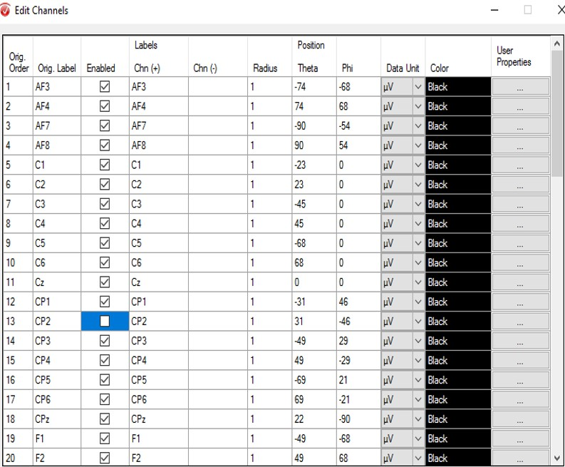
Cycle through the data and identify noisy or dead channels. Noisy channels will have repeating un-patterned, large spikes that are not mirrored in other channels. Dead channels should appear as a flat line. Examine your raw data for bad channels and note which ones you would like to remove. Open the Transformations tab and click Edit Channels. In the pop-up window, uncheck the channels you want to remove, then hit OK.
Cycle through the data and identify noisy or dead channels. Noisy channels will have repeating un-patterned, large spikes that are not mirrored in other channels. Dead channels should appear as a flat line. Examine your raw data for bad channels and note which ones you would like to remove. Open the Transformations tab and click Edit Channels. In the pop-up window, uncheck the channels you want to remove, then hit OK.
Step 2) Change Sampling Rate
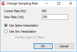
Under the Transformations tab, click Change Sampling Rate. In the pop-up window, insert 250 as your new sampling rate. Select Use Spline Interpolation and click OK.
Under the Transformations tab, click Change Sampling Rate. In the pop-up window, insert 250 as your new sampling rate. Select Use Spline Interpolation and click OK.
Step 3) Re-Reference
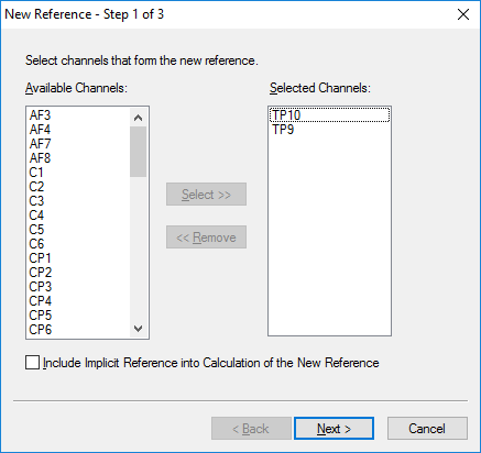
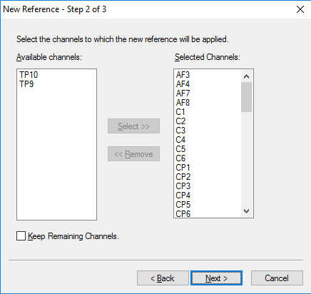
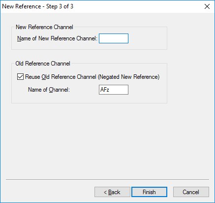
Under the Transformations tab, click Channel Reprocessing. Select New Reference. In the first pop-up window, select the left and right mastoid, M1 and M2 or TP9 and TP10, depending on your data set. Add them to the column on the right. All other channels should remain in the left-hand column. Hit Next. In the next window, add all channels except M1 and M2 (or TP9 and TP10) to the right-hand column. Hit Next. In the third window, hit Finish.
Under the Transformations tab, click Channel Reprocessing. Select New Reference. In the first pop-up window, select the left and right mastoid, M1 and M2 or TP9 and TP10, depending on your data set. Add them to the column on the right. All other channels should remain in the left-hand column. Hit Next. In the next window, add all channels except M1 and M2 (or TP9 and TP10) to the right-hand column. Hit Next. In the third window, hit Finish.
Step 4) Data Filtering
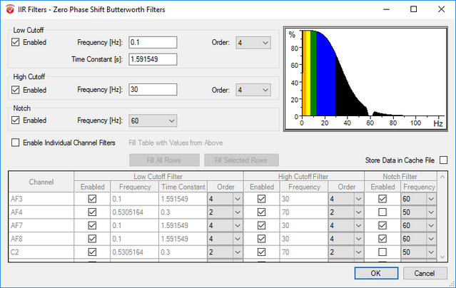
Under the Transformations tab, click Data Filtering and select IIR Filters. Enable the Low Cutoff and insert 0.1 as the frequency. Enable the High Cutoff and insert 30 as the frequency. Enable the Notch and select 60 as the notch frequency. Hit OK.
Under the Transformations tab, click Data Filtering and select IIR Filters. Enable the Low Cutoff and insert 0.1 as the frequency. Enable the High Cutoff and insert 30 as the frequency. Enable the Notch and select 60 as the notch frequency. Hit OK.
Step 5) Segmentation
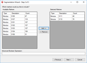
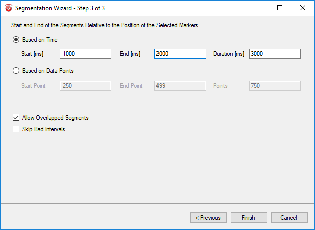
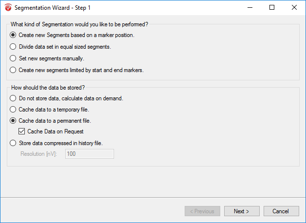
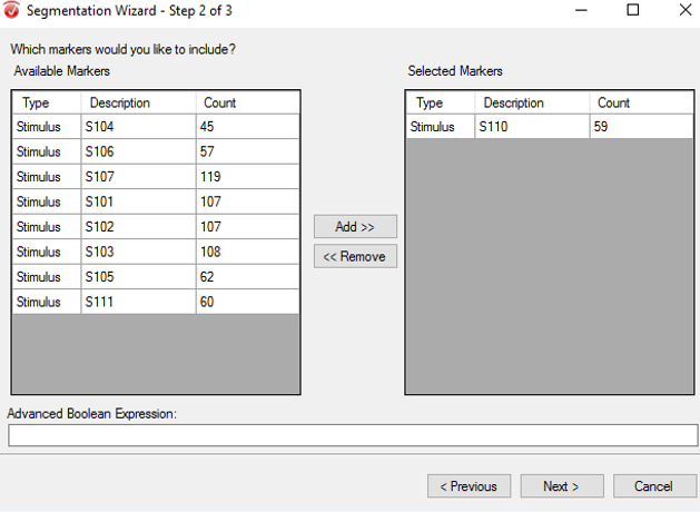
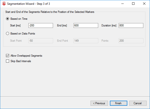
The purpose of segmentation is to extract the 'hits' and 'misses' of the experiment from the remainder of the data collected. Under the Transformations tab, click Segmentation. In the first window, select Create new Segments based on a marker position. Select Cache data to a permanent file. Hit Next. In the next window, select the markers of interest, S 110 and S 111 in this paradigm, add them to the right-hand column, then click Next. In the third window, select Based on Time and insert -1000 in the start box and 2000 in the end box. NOTE: This window size is used independent of the length of the segments/epochs you are interested in. The segment length of 3000 ms chosen here is to facilitate the ICA algorithm. Click Finish.
The purpose of segmentation is to extract the 'hits' and 'misses' of the experiment from the remainder of the data collected. Under the Transformations tab, click Segmentation. In the first window, select Create new Segments based on a marker position. Select Cache data to a permanent file. Hit Next. In the next window, select the markers of interest, S 110 and S 111 in this paradigm, add them to the right-hand column, then click Next. In the third window, select Based on Time and insert -1000 in the start box and 2000 in the end box. NOTE: This window size is used independent of the length of the segments/epochs you are interested in. The segment length of 3000 ms chosen here is to facilitate the ICA algorithm. Click Finish.
Step 6) ICA
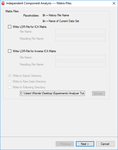
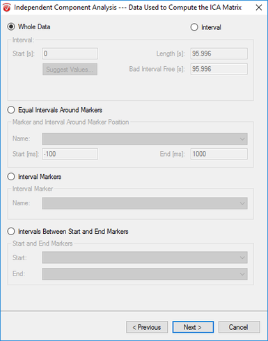
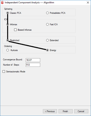
Under the Transformations tab, click ICA. In the first window, uncheck both Write LDR options and select Write to Export Directory. Hit Next. In the next window, hit Enable All, select Number of Enabled Channels, and hit Next. In the third window, select Whole Data and unselect all other options before clicking Next. In the last window, select Classic PCA, Infomax, Assessed, and Energy. Unselect Semiautomatic Mode, and hit Finish.
Under the Transformations tab, click ICA. In the first window, uncheck both Write LDR options and select Write to Export Directory. Hit Next. In the next window, hit Enable All, select Number of Enabled Channels, and hit Next. In the third window, select Whole Data and unselect all other options before clicking Next. In the last window, select Classic PCA, Infomax, Assessed, and Energy. Unselect Semiautomatic Mode, and hit Finish.
Step 7) Inverse ICA
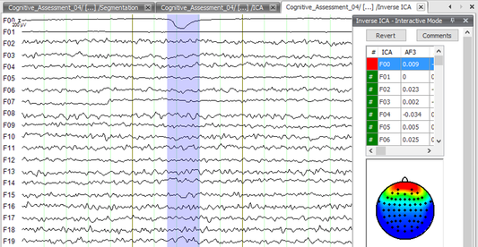
Under the Transformations tab, click Inverse ICA. In the pop up window, select Semiautomatic Mode and press OK. You will now see a screen similar to the one presented below. Scroll through the data until you find blinks - dips in the data as seen below (In the F00 channel). Note the channel(s) that seem to be affected by the blink. Next, select these channels in the table above the topographic map and examine the map for each channel. Those channels affected by the blinks will by highly positive (red) over the frontal lobe and highly negative (green and blue) elsewhere. This is a good way to double check that the channel(s) you originally observed to be affected by blinks truly are demonstrating blink characteristics. So take for example the data presented in the screenshot below; the only channel that appears to be affected by blinks is F00. F00 is selected in the table above the topographic map and the map is showing classic blink activity. When you’re satisfied that you’ve caught all of the channels displaying blinks, click Finish.
Under the Transformations tab, click Inverse ICA. In the pop up window, select Semiautomatic Mode and press OK. You will now see a screen similar to the one presented below. Scroll through the data until you find blinks - dips in the data as seen below (In the F00 channel). Note the channel(s) that seem to be affected by the blink. Next, select these channels in the table above the topographic map and examine the map for each channel. Those channels affected by the blinks will by highly positive (red) over the frontal lobe and highly negative (green and blue) elsewhere. This is a good way to double check that the channel(s) you originally observed to be affected by blinks truly are demonstrating blink characteristics. So take for example the data presented in the screenshot below; the only channel that appears to be affected by blinks is F00. F00 is selected in the table above the topographic map and the map is showing classic blink activity. When you’re satisfied that you’ve caught all of the channels displaying blinks, click Finish.
|
Step 8) Topographic Interpolation
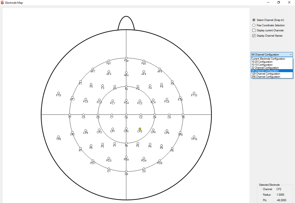
In the Transformations tab, click Topographic Interpolation. In the pop-up window, select Interpolation by Spherical Splines, Default Lambda, and Keep Old Channels. In the table, insert the names of the channels you deleted in the Edit Channels phase by selecting them in the Select from Map option. When you’re done, click OK. |
Step 10) Condition Segmentation
Now you must segment your data into the different conditions of your study (e.g. successful hit, missed target). Under the Transformations tab, click Segmentation. In the first window, select Create new Segments based on a marker position. Select Cache data to a permanent file. Hit Next. In the next window select the markers of interest (S110 for hits or S111 for misses) and add them to the right-hand column then click Next. In the third window select Based on Time and insert -200 in the start box and 600 in the end box. Note: The segment length here is dependent of the ERP component of interest. For the P1/N1 a segment length of 600 ms is all you need: -200 to 400 ms. For the FRN/RP 800 ms, -200 to 600 ms, for the P300 you may need a segment length of 1000 ms: -200 to 800 ms. Click Finish. This step should be repeated for each marker of interest (hit marker S 110 and miss marker S 111).
Now you must segment your data into the different conditions of your study (e.g. successful hit, missed target). Under the Transformations tab, click Segmentation. In the first window, select Create new Segments based on a marker position. Select Cache data to a permanent file. Hit Next. In the next window select the markers of interest (S110 for hits or S111 for misses) and add them to the right-hand column then click Next. In the third window select Based on Time and insert -200 in the start box and 600 in the end box. Note: The segment length here is dependent of the ERP component of interest. For the P1/N1 a segment length of 600 ms is all you need: -200 to 400 ms. For the FRN/RP 800 ms, -200 to 600 ms, for the P300 you may need a segment length of 1000 ms: -200 to 800 ms. Click Finish. This step should be repeated for each marker of interest (hit marker S 110 and miss marker S 111).
|
Step 11) Artifact Rejection
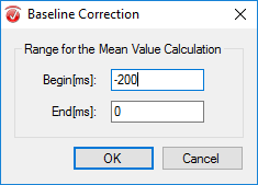
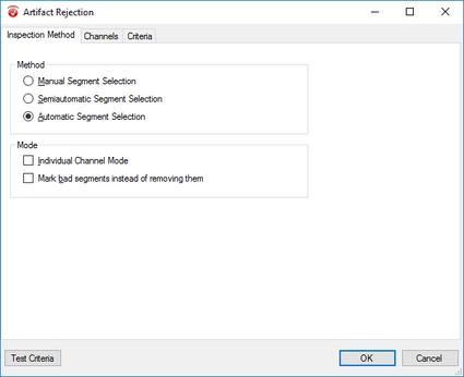
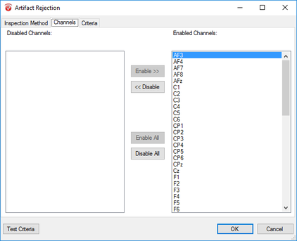
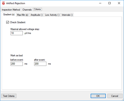
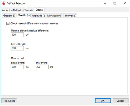
Click Artifact Rejection under the Transformations tab. From here, follow the following four steps: I. In the pop-up window select Automatic Segment Selection under the Inspection Method tab. Uncheck all other options under this tab. II. Now, in the same window, move to the Channels tab. Here, select Enable All. III. Move to the Criteria tab and in the Gradient sub-tab select Check Gradient and insert 10 into the Maximal Allowed Voltage text box. In the Before Event space insert 200. Do the same in the After Event text box. IV. Now move to the Min-Max sub-tab and select Maximal Allowed Absolute Difference. In the following text box insert 100. In the Interval Length text box insert the length of your segment (e.g. 800ms: see above). In the Before Event space insert 200. Do the same in the After Event text box. Finally, finish up artifact rejection by clicking OK. |
Step 12) Evaluating Data
Right click the Artifact Rejection Node and select Operation Info. The new pop-up window should show the number of kept segments, removed segments as well as the percentage of data removed from each specific electrode. Ideally the number of Removed segments will be no more than 10% of the Total number of segments. However the proportion of acceptable removed to total data may vary depending on your labs protocol.
Right click the Artifact Rejection Node and select Operation Info. The new pop-up window should show the number of kept segments, removed segments as well as the percentage of data removed from each specific electrode. Ideally the number of Removed segments will be no more than 10% of the Total number of segments. However the proportion of acceptable removed to total data may vary depending on your labs protocol.
Step 14) Data Export
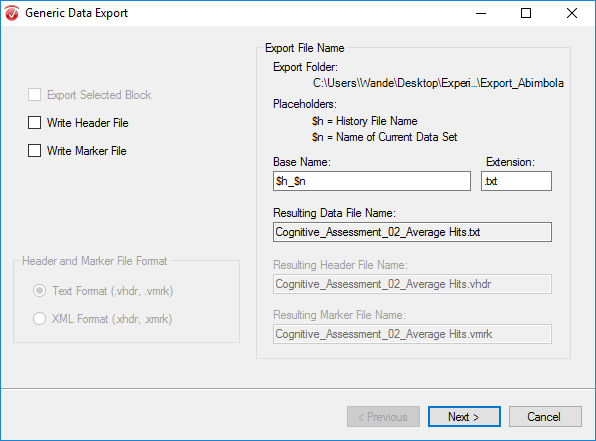
Go to the Export tab and select Generic Data.
Go to the Export tab and select Generic Data.
In the pop-up window, insert $n_$h as the Base Name. Uncheck Write Header File and Write Marker File. Click Next.
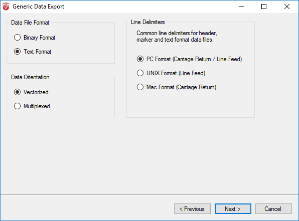
In the next window select Text Format, Vectorized, and PC Format. Click Next.
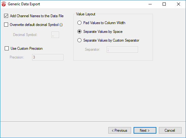
In the third window, select Add Channel Names to the Data File and Separate Values by Space. Click Next.
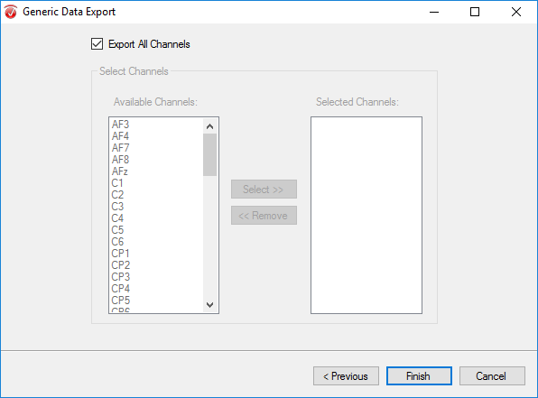
Finally, select Export All Channels and hit Finish.
Step 15) Grand Average
Conduct this step when you have completed All of the previous steps for each of your participants. In the Transformations tab, go to the result evaluation drop down menu. Select Grand Average. In the Input History Nodes and Output Files table, put the name of the all conditions in both columns. Add All channels to the column on the right (Selected Files). Ensure Primary History Files is selected, along with Select Individual History Files.
Conduct this step when you have completed All of the previous steps for each of your participants. In the Transformations tab, go to the result evaluation drop down menu. Select Grand Average. In the Input History Nodes and Output Files table, put the name of the all conditions in both columns. Add All channels to the column on the right (Selected Files). Ensure Primary History Files is selected, along with Select Individual History Files.
Step 16) Final Export
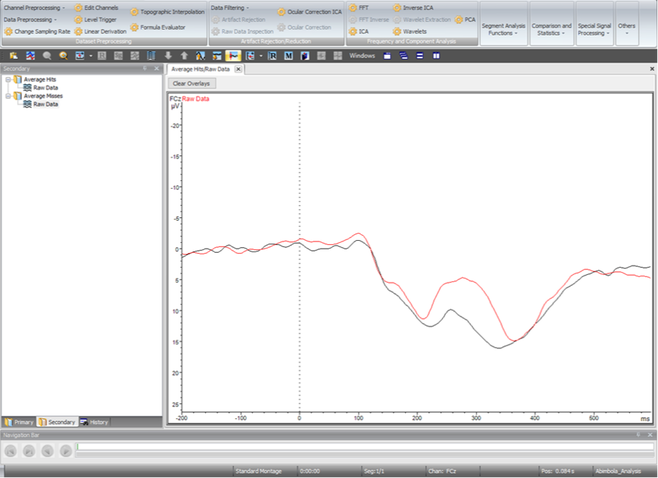
The averaged data should now exist in the Secondary tab in Analyzer. The raw averaged data for all conditions should be visible, and can be combined to create graphs of average amplitudes at each electrode (As seen below). To export the averaged data select Raw Data of a condition, navigate to the Export tab, and select Generic Data as before.
The averaged data should now exist in the Secondary tab in Analyzer. The raw averaged data for all conditions should be visible, and can be combined to create graphs of average amplitudes at each electrode (As seen below). To export the averaged data select Raw Data of a condition, navigate to the Export tab, and select Generic Data as before.
Statistical Analysis
In the past we have quantified the FRN as either the maximal negativity on the difference waveform in a window centred around the peak of the grand average difference waveform (e.g., between 200 and 400 ms) or as the mean over a shorter window (peak +/- 20 ms) also centred on the peak of the grand average difference waveform. In terms of topographies, we typically used the "peak topography" generated from the peak detection process as opposed to the topography of the peak difference of the grand average difference waveform.
In the future, we hope to move away from this and instead use and promote the use of confidence intervals plotted for each time point of the grand average difference waveform for each effect of interest.
In the future, we hope to move away from this and instead use and promote the use of confidence intervals plotted for each time point of the grand average difference waveform for each effect of interest.
